
What could a megakernel win on a Mac?
A persistent GPU kernel can remove gaps between operations. We measured how much room that leaves on Apple silicon: about 1.1 ms per decode step on an M5 Max, with a very different payoff for small and large models.

Chapters
A GPU can spend part of its time waiting for its next piece of work. That is an uncomfortable thought when you are watching a local language model produce an answer, token by token, on an expensive computer.
Megakernels tackle those gaps by keeping more of a model's forward pass inside a persistent GPU program. Work such as Hazy Research's “Look Ma, No Bubbles!” makes the idea tangible: changing how work is scheduled can matter as much as accelerating an individual operation.1
For a Mac running MLX, we wanted to ask an earlier question. Before building a megakernel, how much time could one plausibly recover? If most of a decode step is already spent reading weights at close to the available bandwidth, a better schedule cannot make those bytes disappear.
Separating the journey from the loading
Consider a simple model of each generated token's cost:
The second term is the time spent streaming weights. The first collects work that does not scale with their byte count: scheduling, cache updates, sampling and other per-step work. It is an estimate of the room for optimisation, not a stopwatch aimed specifically at kernel-launch gaps.2
To separate the terms, we used a useful pair of models. Qwen3 0.6B and 1.7B have the same measured decode graph, with 821 primitives.3 Their weights differ in size, so the change in step time gives us a way to estimate the marginal cost of streaming those weights without also changing the graph's operation count.
On an M5 Max with 128 GB, the pair took 1.629 and 2.694 milliseconds per token. The implied marginal bandwidth was 595 GB/s, about 97% of the nominal 614 GB/s.4 There was little unused bandwidth left for that part of the work.
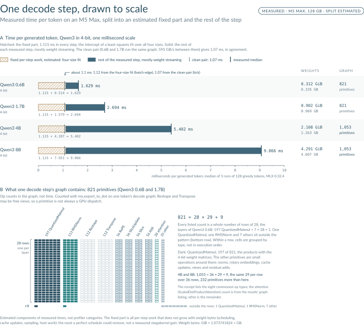
Decode time per token on an M5 Max, drawn to scale: the estimated fixed per-step work stays about 1.1 ms while the rest of the step, mostly weight streaming, grows with model size. The step times are measured; the split uses the four-size fit's intercept, agrees with the clean pair, and is neither a profiler measurement nor a measured megakernel gain.
The same fixed cost can be a large or small opportunity
The clean pair gave a fixed-cost estimate of 1.07 ms. A fit across all four tested sizes gave 1.12 ms. Those estimates agree closely enough to describe the result as about 1.1 ms per decode step.
With the four-size fit, the fixed part represents about 68% of the Qwen3 0.6B step. For 8B, it is about 12%. The absolute cost is similar; the part of the wait it occupies is not.
That distinction changes which optimisation is worth pursuing. A small model can spend much of its step doing work around the weight stream. A larger model spends more of it moving the weights themselves. A persistent kernel has a more promising ceiling in the former case.
The ceiling is generous. It assumes the fixed part can be removed, although some of that work is necessary computation. We did not build a megakernel here, and the estimated share is not a measured speedup from one.
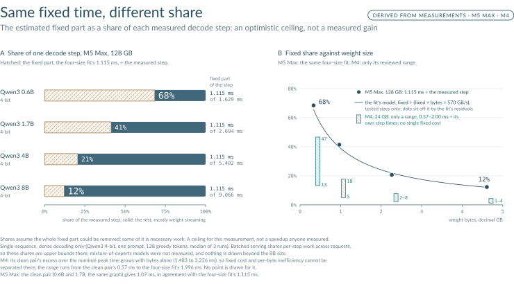
Fixed-cost shares fall from 68% for the smallest model to 12% for the largest, showing why the same optimisation has different value. Both come from the four-size fit's fixed part and measured step times; they are optimistic ceilings for single-sequence dense decoding, not measured gains, and the M4 gives only a range.
Could the model predict an unseen measurement?
A line fitted after every run can look persuasive without teaching much. We therefore wrote down and hashed a prediction before running the 8B case:
It predicted 8.8 ms per token, with a band of 7.5–10.1 ms. The measured result was 9.07 ms, inside that band without refitting.
The recorded timeline is consistent with the prediction preceding the run. It was not separately pushed before the measurement, so this is a recorded prediction rather than an independently verified preregistration.
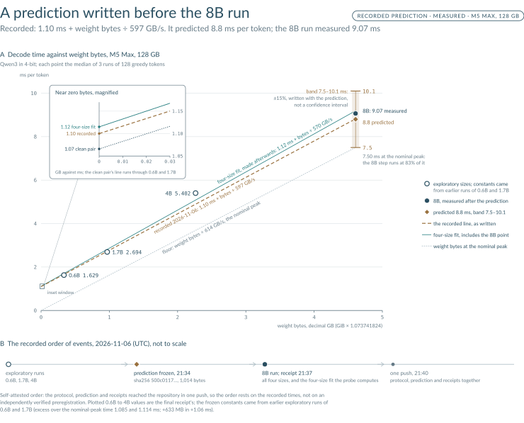
Decode time against weight bytes shows the fitted intercepts and the recorded 8B prediction band beside the later measured point, on the M5 Max. The band is the tolerance written with the prediction, not a confidence interval, and the order of events is self-attested.
For this dense 8B model, stock decoding already reached 83% of the machine's nominal peak bandwidth. That does not make further optimisation pointless. It tells us where an explanation of a large speed claim would need to look: less traffic, a different workload, or a larger source of overhead than this test exposed.
A second Mac gave a less tidy answer
The experiment used MLX 0.32.4 and 4-bit Qwen3 models at 0.6B, 1.7B, 4B and 8B. We measured greedy generation from one prompt for 128 tokens and reported medians of three runs. Alongside the M5 Max, we ran the panel on an M4 with 24 GB.
On the M4, the estimators did not agree closely enough to justify a single fixed-cost number. The reviewed range was about 0.6–2.0 ms. The excess time in the clean pair was not constant, so we could not separate fixed overhead from inefficiency that grew with the bytes moved.
A simple model can be useful on one machine and insufficient on another. Keeping the M4 range is more informative than forcing both computers onto an equally neat line.
These measurements concern single-sequence, dense-model decoding. They do not establish the opportunity for mixture-of-experts models. Batched serving also shares per-step work across requests, so the fixed-cost shares here are generous bounds for that setting.
We explored a different way to reduce weight traffic in Fewer experts, faster answers on a Mac?, where reducing the active experts changed both generation speed and answer quality.
A smaller experiment before a larger kernel
MLX already offers a way to reduce overhead and fuse work: mx.compile.5 In a small chain of dependent operations, compilation reduced the measured cost per chain step. Each step contains three operations: two multiplies and an add.
| Machine | Plain, µs/step | Compiled, µs/step | Ratio |
|---|---|---|---|
| M5 Max | 3.88 | 0.48 | 8.1× |
| M4 | 4.92 | 0.66 | 7.5× |
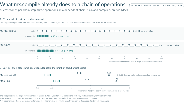
Uncompiled and compiled costs per chain step of three operations show an existing optimisation opportunity without presenting it as a whole-model speedup. A microbenchmark on two Macs; mlx-lm already compiles part of its decoding step.
This is a microbenchmark, not a claim that language-model generation becomes that many times faster. mlx-lm already compiles parts of the model, such as the SwiGLU activation used by Qwen3.6 The useful question is which remaining parts of a particular workload can benefit, not whether a familiar API name has been switched on everywhere.
A full persistent kernel faces another problem: coordination. We found no cooperative-launch facility or device-wide barrier in Metal that guarantees the required threadgroups run together. A kernel implementing its own spinning coordination would need to deal with the absence of that co-residency guarantee. The scheduling problem does not disappear when scheduling moves inside a kernel.7
Conclusion: where a megakernel could help
We measured single-sequence decoding across four dense Qwen3 model sizes on two Macs to estimate the room for a megakernel before building one. Separating weight traffic from per-step work gave a useful model on the M5 Max: its prediction for the later 8B run landed inside the recorded band without refitting.
The clearest result was about 1.1 ms of fixed work per decode step: roughly 68% of the smallest model's decode step, but only 12% of the largest model's. Those are optimistic limits on the opportunity, not gains we achieved. Some of that fixed work is necessary computation, and a megakernel would still have to read the weights.
That gives an engineer a direction. For these small-model workloads, reducing work around the weight stream is worth investigating. For the larger model, moving the weights dominates, so scheduling alone has less room to help. The M4's less tidy result is a reason to make that estimate on the intended machine rather than borrow the M5 Max's ceiling.
Before committing to a persistent kernel, check which remaining operations can benefit from ordinary compilation and fusion. Our mx.compile experiment showed how much that can matter in a dependent chain, although it did not measure a whole-model gain. The useful outcome is a way to choose the next optimisation: measure which part of the wait you can change, and how much of each decode step it actually occupies.
Footnotes
-
Spector, Juravsky and colleagues, Hazy Research, Look Ma, No Bubbles! Designing a Low-Latency Megakernel for Llama-1B, May 2025. Their explanation covers scheduling, overlapping memory loads and synchronisation inside a persistent kernel on NVIDIA GPUs. The accompanying Megakernels repository contains the implementation. ↩
-
Williams, Waterman and Patterson, Roofline: An Insightful Visual Performance Model for Floating-Point Programs and Multicore Architectures. The paper provides background on reasoning from compute and memory-bandwidth limits. Our fixed-cost-plus-weight-traffic equation is an empirical timing model; the fitted intercept and the Mac measurements are our own. ↩
-
Qwen team, Qwen3 Technical Report, May 2025, describes the model family. We used the mlx-community 4-bit conversions: 0.6B, 1.7B, 4B and 8B. The equal primitive counts are from our MLX graph inspection, not a claim from the model report. These links identify the model repositories, not immutable snapshots of our run. ↩
-
Apple's M5 Pro and M5 Max technical specifications list 614 GB/s for the M5 Max configuration with a 40-core GPU; Apple offers 128 GB only in that configuration. We use that vendor specification as the nominal denominator; the fitted marginal bandwidth is derived from our timings. ↩
-
MLX's compilation guide explains graph simplification, operation fusion and compilation caching. The guide source at MLX 0.32.4 preserves the version used here. Compilation can reduce intermediate work; its benefit depends on the graph being compiled. ↩
-
For a concrete source example, mlx-lm 0.32.0's SwiGLU activation is decorated with
mx.compile, and its Qwen3 MLP calls that activation. This illustrates compilation already present within the model, rather than a single switch that compiles the entire generation loop. ↩ -
Apple's guide to porting Metal code to Apple silicon explains shader synchronisation, with the full definitions in the Metal Shading Language specification. In particular,
threadgroup_barrier(mem_device)coordinates threads within a threadgroup and their device-memory accesses; themem_deviceflag does not turn it into a rendezvous across every threadgroup. That scope matters when designing an in-kernel coordination scheme. ↩