
Meet your one-pass AI opponent
Play Connect Four against a 7.8 MB local AI in your browser. A better teacher turned our losing first attempt into a much tougher opponent.
%20scale(.916666667)'%20d='M18.9%202H22l-6.8%207.8L23.2%2022h-6.3L12%2014.6%205.5%2022H2.4l8.2-9.5L2.8%202h6.4l4.5%206.8L18.9%202ZM17.9%2020h1.7L8.2%203.9H6.4L17.9%2020Z'/%3e%3c/svg%3e)
Chapters
Drop a disc into a column and watch the AI make its move. Your opponent is a 7.8 MB model running locally in your browser. It reads the board, gives each legal column a score, and plays its favourite. One forward pass per move, with no search through future positions. In our Chromium test on an M1 Max, it chose a move in about 20 milliseconds.1
Play Connect Four against it. You can go first or let it open. Its column preferences are visible too, so there is something to inspect while planning your revenge.
Games have become an appealing place to explore this style of AI. TypeSafe's
September launch of Jev included a Doom demonstration built around fast,
structured decisions. Independent projects such as jevlike and open-jev
explore related ideas in Doom and chess.2
Convai Innovations' Laya offers open-source code and model weights for typed decisions without generating text. Community demos put it behind falling blocks in Tetris and the next turn in Snake. Familiar games make an abstract interface rather fun to watch.3
The attraction of these decision models is easy to see in a game. The application knows the current state and the available actions. The model's job is to judge which action to take. That is a small, useful place to put learning inside ordinary software.
Our previous OnePass article explored that idea with a Swedish form specialist. We wanted to try it in a setting where the consequences are more visible, and where the reader can join in. This is a new model trained for Connect Four, using open code; it does not use TypeSafe's Jev model or API, or Laya's weights.
Our first attempt was an easy opponent. Two days later, a revised version won about nine in ten games against a four-move search bot under our test rules. Getting there taught us more about what to teach the model than its small download might suggest.
For a Connect Four product, a search-based opponent would be a sensible choice. The four-move bot is our simple benchmark. The exact solver we use as a teacher can play perfectly and already has a browser version. Its WebAssembly module and JavaScript total about 1.29 MB, including its opening book, compared with 7.82 MB for our model alone, before adding the model's runtime.4
There is also a difference in when the work happens. The solver searches during play, and the amount of search depends on the position. Our model uses the same fixed-size network evaluation for each move, giving it a more predictable amount of computation.5
To make that variation concrete, we timed a native build on an M5 Pro. Across 200 positions eight moves into a game, scoring every legal column took a median 0.84 seconds, with the slowest at 16.6 seconds. Its opening book can make the very first moves much cheaper. These measurements illustrate variable search cost; they are not a matched speed test against the browser model.6
For the player, the model's advantage is a quick, predictable turn time throughout the game. It runs the same fixed-size computation in the opening, middle game and endgame, with about 20 milliseconds per move measured in our M1 Max browser test.1
We chose Connect Four to explore how a model learns decisions. A solved game lets us check its choices against exact answers. In other games or applications, a practical exact solver may not exist. Teaching examples could instead come from expert play, a slower planning system or observed outcomes. This board gives us a clear place to start.
A board, seven options, one decision
Connect Four has a small vocabulary: seven columns, six rows, and four discs in a line to win. The next move is a choice among the columns that are not full. That fits the OnePass interface neatly.
The model receives a 44-byte description: whether it is the first or second
player, followed by 42 cells from its own point of view. A cell is empty, mine or
theirs. The available actions are short strings such as column 3 and
column 7. One evaluation of the network returns a score for each legal
action.7
The application still checks legality, drops the disc and detects a win. The model supplies the playing strategy. It does not expand a tree of future moves, call a solver or generate a written answer before choosing.
This is a small transformer from the same architectural family as our form specialist, scaled up to 7.4 million parameters, with new weights trained for the game. It builds on the open Cua-S1 scorer, whose option-attention head comes from the jevlike project.8
The bars in the demo make that narrow interface visible. They show relative preferences derived from the model's scores, not measured chances of winning. They cannot tell us why it likes a move, but they let us see what it chose over the alternatives.
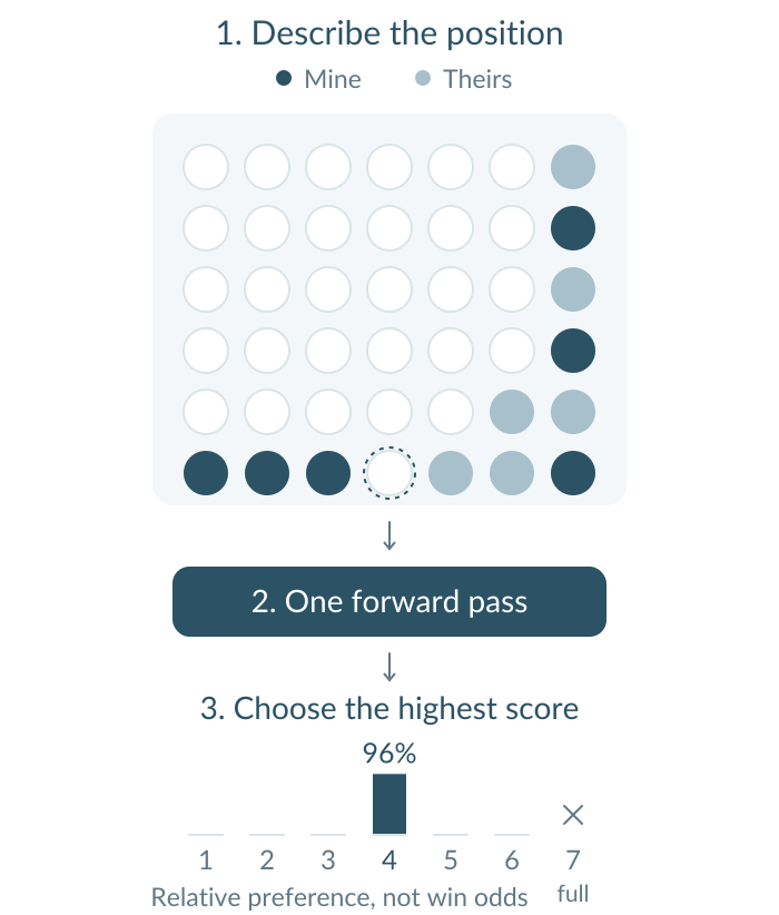
The image above shows a simple position to make the interface concrete. Column 7 is already full, so it is not an option. The outlined space in column 4 completes the row. The preferences shown come from running the released int8 model on this board with native ONNX Runtime. The position and output scores are available to inspect.
Our first AI player was an easy opponent
The first attempt, concluded on 24 September, had about 0.7 million parameters. It almost never beat a simple bot that searched four moves ahead. On the later comparison protocol, it won just six of 200 games against that bot.
Its education had a large hole in it. The exact solver we initially used was practical only near the end of a game, with at most 16 empty cells. Most of the training positions were random fills of those late boards. The model could see what a good ending looked like without getting exact instruction for much of the opening and middle game.9
Adding a small set of opening games labelled by the four-move bot did not produce a clear improvement. We had widened the lesson, but the teacher still had a limited view. A plausible next move from a shallow search is not the same thing as knowing which moves preserve a win.
There was another warning: a respectable score on individual positions did not turn into good games. A player has to carry its advantage from one decision to the next. We needed to improve the training and keep playing complete matches to see whether it helped.
Teaching v2 the whole game
Connect Four gives us an unusually helpful teacher: it is a solved game. An exact solver can tell whether a move preserves a forced win, a draw or a loss, assuming perfect play afterward. We do not have to guess whether a training label is good.
For the second attempt, we used Benjamin Rall's MIT-licensed connect-four-ai to label positions throughout the game. We also used the MIT-licensed TonyCWang/ConnectFour dataset, which already contains exact labels from Pascal Pons' solver.
The available pool grew to roughly 42 million positions: 41.6 million from the dataset and another 513 thousand generated from games between players of different strengths. Those weaker players matter. A human opponent will not always follow the teacher's preferred line, and the model needs examples of what happens after a mistake too.
We also made the board easier to read. Instead of a longer text grid and move history, each cell had a fixed place in a compact description, always from the next player's perspective. In an early diagnostic run, even a model at the old size became much more sensitive to which player owned each disc. That gave us reason to keep working on the recipe before blaming the basic architecture.
Teach how moves compare
We changed the target as well. Instead of teaching only one correct column, we trained the model to rank all legal moves: preserve a win before settling for a draw, prefer a quicker win, and delay an unavoidable loss.
Several columns can be good. Treating one as the right answer and the others as wrong discards information the solver already has. The new target teaches those relationships across the legal options. In the training comparisons, this ranking target also outperformed a target that treated all value-preserving moves equally.10
Then we increased capacity. A medium model and the larger version had very similar position-level accuracy, but their game results were far apart. The larger network was worth keeping because it played better, not because its validation score looked dramatically different.10 Further training also lifted the full-precision model's game score against a two-move search bot from 64.3% to 90.5%.11
The improvement came from a revised training recipe, not a larger model alone. Labels, examples, input representation, target and capacity all changed. The public recipe includes the intermediate comparisons.9
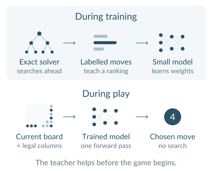
The solver explores what could happen next to produce the teaching signal. The student learns from those answers. Later, it can choose a move without repeating the search. The teacher's certainty does not transfer intact: the student is an approximation, and we still have to find out how well it plays.
What changed on the board?
We fixed the game-test rules before training the second version. Each match contains 200 games from an empty board, with the first player alternating. On every turn, both players have a 5% chance of making a uniformly random legal move. This introduces variation instead of replaying the same deterministic game, although some games still repeat. A win earns one point, a draw half a point.12
Here are the primary results. The two search bots look four or six moves ahead, counting one player's turn as one move. The learned players do no search. The browser download uses int8 quantisation: most weights are stored as eight-bit integers instead of 32-bit floating-point numbers, making the file smaller.
| Opponent | First version | v2, full precision | v2, int8 browser file |
|---|---|---|---|
| Four-move search bot | 3.0% | 91.5% | 90.5% |
| Six-move search bot | 2.0% | 89.25% | 87.75% |
Percentages are game scores under the rules above. The int8 results evaluate the same compressed file distributed to browsers, using native ONNX Runtime for these matches.13
The downloadable model beat the four-move search bot in 181 of 200 games. The full-precision checkpoint won 183. Keeping those results separate matters: shrinking a model for delivery is another change to evaluate, not just a smaller download.
For reference, the exact solver scored 89% against the four-move bot under the same rules. That is lower than either v2 point estimate, but it does not make our model better than the solver. The solver also suffers the forced random moves, and these are finite samples. In a direct match against it, the full-precision model scored 47.5%, roughly even under those noisy rules. That is not a claim of perfect play.13
Separate browser-arena testing produced a satisfying 200-0 against v1. That arena uses random opening moves rather than the 5% override throughout the game, so it is a different test. It contained 83 distinct games, not 200 unique contests. It is a useful demonstration of progress, rather than a rating against human players.1
A position-by-position check offers another view. On 17 325 test positions, the full-precision and int8 files chose the same column 98.2% of the time. Each preserved the position's win/draw/loss value in about 98.7% of positions.14 Test positions with at least 12 discs were held out from training; earlier positions could overlap. The remaining mistakes still matter: a game gives a player several chances to throw away a good position.15
The browser release runs on WebAssembly, which lets a web page execute compiled code locally in the browser. Once the model and runtime have downloaded, no server is needed to score a move. The 7.8 MB figure is for the model file downloaded from Hugging Face (excluding the browser runtime).
See the code: training on Apple Silicon
We did the training on Apple Silicon. We trained the released model with MLX on an Apple M5 Pro, using the labelled boards and move rankings described above. The training run had two stages, with a lower learning rate in the second.
| Training run | Value |
|---|---|
| Model size | 7.4 million parameters |
| Training steps | 6 000 + 12 000 |
| Batch size | 1 024 board positions |
| Samples drawn | 18.4 million |
| Input tokens | 812 million byte tokens |
| Training time | About two hours |
Each board description uses 44 byte tokens. The token total also includes the column labels, which the MLX trainer encodes once per batch and shares across its boards.16 Positions can be sampled again, so the sample count does not represent unique boards.9
Our Connect Four AI recipe follows the whole process: prepare the labelled data, exclude test positions, train, play the evaluation matches, and export the model. It includes the protocol and result files behind the numbers in this article.
The MLX trainer runs the same model and training recipe as the toolkit's PyTorch implementation. It saves portable weights and checks the saved model against the PyTorch version. The export script then uses that version to produce an ONNX file. We apply ONNX Runtime's dynamic int8 quantisation, reducing the model file from 29.7 MB to 7.8 MB, and evaluate the quantised file again before putting it in the browser. This needs no retraining or calibration dataset: the weight matrices and embedding table use eight-bit storage, while components such as layer norms and biases stay in float32.17
The onepass-web repository contains the other half: the game, board encoding and browser runtime. Training uses MLX; the browser uses ONNX Runtime Web with WebAssembly. A player needs neither MLX nor an Apple computer to try the result.
Conclusion: your move
The useful step from v1 to v2 was learning to teach the whole decision. That meant examples from across the game, including mistakes, and a target that showed how the legal moves compared. A larger model helped, but complete games told us whether the changes had made a better opponent.
This is the part we hope other builders will take further. A puzzle hint, a turn-based opponent, or a character choosing its next action could all be interesting places to try a small decision model. The same interface can sit inside a browser game or a native app: game code supplies the state and legal actions, the model scores them, and the game carries out the choice.
Our Connect Four weights are a specialist for this board. A different game would need its own examples and evaluation, perhaps with a solver, an existing game bot or recorded expert moves as the teacher. The open tools are there for that next experiment.
For us, this is a starting point too. There are many more decisions worth teaching, and many fun games to try. A game is a lovely way to experience AI, discover what a model has learned, and give a human player a fun challenge.
For now, there is a seat on the other side of the board. Can you beat our model?

Footnotes
-
The public demo documentation, implementation and model card document the demo, available models and arena rules. The standard release uses WebAssembly. ↩ ↩2 ↩3
-
TypeSafe introduced Jev on 15 September 2026, with Doom among its launch demonstrations. The independent jevlike project includes Doom and chess experiments; daseinlabs/open-jev demonstrates local option scoring with Gemma and a Doom action menu. These are examples of related interfaces, not evidence that the models share TypeSafe's architecture, training method or level of playing strength. ↩
-
Laya's model card describes its ModernBERT-family encoders and decision head; code and weights are Apache-2.0 licensed. It shares the structured-decision pattern with our specialist, with different architecture and training. The Tetris implementation gives Laya a shortlist of placements ranked by a heuristic. The Snake demo supplies planner features and, by default, a visible safety layer that can override a proposed move. These are examples of integrating model decisions into games, not a comparison of unaided playing strength. ↩
-
The exact connect-four-ai solver is separate from our depth-limited benchmark bot and has its own playable browser demo. In the published
connect-four-ai-wasm1.0.0 package, the.wasmfile is 1 260 614 bytes and its JavaScript wrapper is 26 817 bytes, totalling 1 287 431 bytes. The module contains the default depth-eight opening book. Our int8 model file is 7 816 833 bytes, about 6.1 times that total. These are uncompressed file sizes, excluding both frontends and the model's ONNX Runtime, not network-transfer sizes, memory use or a speed comparison. The size receipt records the versioned downloads, byte counts and hashes. ↩ -
The solver implementation checks its opening book and otherwise searches the game tree. The model export fixes the board input at 44 bytes and the option input at seven eight-byte slots, masking illegal columns. Its computation does not expand with the depth of a position's possible continuations. Fixed computation does not guarantee identical wall-clock latency; this is not a timed solver-versus-model comparison. ↩
-
The public timing receipt and measurement script use a native Rust build of
connect-four-aiat28a112aon an 18-core Apple M5 Pro. Each position is solved on one thread, with eight independent positions in parallel. The search cache is cleared before each position, outside the timed region; startup and downloads are also outside it. A seeded sample of 200 UCI eight-ply positions took a median 839.33 ms, a 95th percentile of 4 854.392 ms and a maximum of 16 572.782 ms to score all legal columns. The depth-eight opening book is enabled, but evaluating each possible move from these positions reaches the ninth ply, beyond the book. This does not measure the first move from an empty board or a browser solver's latency. The receipt also includes six Pascal Pons reference sets, showing substantial variation across positions. The model's roughly 20 ms figure comes from a separate Chromium/WebAssembly check on an M1 Max; no cross-runtime speedup ratio is inferred. ↩ -
The public input contract specifies the 44-byte perspective board, legal columns and byte encoding. ↩
-
The toolkit's third-party notices credit Cua-S1 and jevlike. The game model uses the 8-layer, 256-wide configuration of the same scorer, with 7.38 million parameters. ↩
-
The published recipe documents the data, targets, model sizes and training schedule. Verification of the teacher also used Pascal Pons' public test positions and the UCI Connect-4 database, contributed by John Tromp and licensed CC BY 4.0. The external dataset's labels were sampled and re-solved to check agreement with the teacher. ↩ ↩2 ↩3
-
The public recipe describes the target and capacity comparisons. At 6 000 steps, the 3.28-million-parameter and 7.38-million-parameter models scored 63% and 89.5% against the four-move bot under the fixed protocol. Their value-preserving accuracy on the fixed position set was 97.48% and 97.77%. These were intermediate checkpoints, not the final release: game results and position results. The original-size diagnostic run was exploratory and preceded the final training/evaluation exclusions. ↩ ↩2
-
Against the two-move bot, the full-precision model's game score rose from 64.25% at the intermediate checkpoint to 90.5% in the final checkpoint. Both matches use 200 games, seed 2026 and the 5% random-move rule. Game score counts a win as one point and a draw as half a point. The final score happens to equal the int8 model's 90.5% against the four-move bot in the later table; those are separate matches with different opponents and model files. ↩
-
The frozen test protocol defines the opponents and random-move rule. The headline matches use seed 2026. Two further seeds give full-precision scores of 89.25% and 90.75% against the four-move bot; this is evidence for this opponent and protocol, not a universal strength rating. ↩
-
Raw results: v1, full-precision v2, int8 v2, and the solver reference. The reported 95% Wilson intervals for the four-move matchup are 85.6-93.8% for int8 v2, 86.8-94.6% for full precision, and 83.9-92.6% for the solver. The direct solver match was not run for the int8 file. ↩ ↩2
-
The paired full-precision/int8 receipt and comparison script evaluate both ONNX files on the same 17 325 positions with ONNX Runtime 1.30.0's CPU provider on an M1 Max. They chose different columns in 321 positions, agreeing in 98.15% to the receipt's precision. Both value-preserving rates round to 98.72%; this is aggregate agreement, not identical choices or proof of equal playing strength. Thirteen changed choices also changed whether the position's win/draw/loss value was preserved. The median gap between the full-precision model's top two scores on changed-choice positions was 0.0044. Counts may vary slightly with integer kernels on other CPUs. The receipt records hashes for both model files, including the released int8 file used here. ↩
-
The first row of the full-precision results records the position metrics. The protocol excludes evaluation positions and their mirrors from training for positions with at least 12 discs on the board. Value preservation asks whether a winning position remains winning, or a drawable one remains drawable, assuming perfect subsequent play; it is not the model's probability of winning a game. ↩
-
Calculated from the 18 000-step schedule, batch size 1 024 and the MLX forward pass: 18 432 000 boards × 44 context tokens = 811 008 000 board-input tokens. Each step also encodes seven shared eight-byte column labels, adding 18 000 × 7 × 8 = 1 008 000 option tokens. Total: 812 016 000 byte tokens through the training input encoders, rounded to 812 million. This excludes evaluation and does not count backward passes or repeated processing through transformer layers as additional tokens. These fixed byte inputs are not directly comparable to word-piece tokens in language-model training. ↩
-
The recipe calls
quantize_dynamicwithweight_type=QuantType.QInt8. This is post-training quantisation: weights are converted after training, and ONNX Runtime calculates activation scales at run time. Inspection of the pinned int8 file shows 39 signed-int8 weight matrices and a uint8 embedding table, about 99.4% of its stored parameter values. Layer norms, biases and positional values remain float32, as do the attention matrix multiplications between activations. Those remaining values, scales and graph data help explain why the file shrinks by about 3.8 times rather than exactly four. The file sizes are recorded in the pinned model card; playing results for the quantised file are shown separately in the table above. ↩