
One millisecond to make a move
Our Connect Four AI already knew how to play. A small WebGPU runtime made its moves faster and its download lighter. Then a human paused to think.
%20scale(.916666667)'%20d='M18.9%202H22l-6.8%207.8L23.2%2022h-6.3L12%2014.6%205.5%2022H2.4l8.2-9.5L2.8%202h6.4l4.5%206.8L18.9%202ZM17.9%2020h1.7L8.2%203.9H6.4L17.9%2020Z'/%3e%3c/svg%3e)
Chapters
Thirteen milliseconds is not a long wait for an opponent. Most of us need longer just to notice whose turn it is. But a small AI model arrives with more than its learned weights: the browser also needs the software that runs them. That code must be downloaded, started and fitted around everything else the page is doing.
In our first Connect Four article, we trained a small model to score the available columns in one forward pass, without searching future positions. This time we kept the trained model and worked on its runtime. Could we make a local decision cheaper to deliver, as well as quicker to make?
On an idle M5 Pro in Chrome, warm moves with the 7.8 MB int8 model file took about 1 ms with our WebGPU runtime, compared with 12.7 ms using ONNX Runtime Web's single-threaded WebAssembly backend. The runtime code fell from 14.3 MB to 37 KB, before network compression. The model download is separate.1
The small numbers were satisfying. The more useful lesson arrived when a human stopped to think between moves.
Try the speed comparison in your browser. Play a game, then run the benchmark. Its comparison table brings download size, start-up and move timings together, highlighting the best value in blue and the worst in red. The spread chart shows how much the turn times vary on your machine.
A smaller engine for the same player
A runtime takes the model's stored numbers and carries out its calculations. ONNX Runtime Web is a general tool for doing that across many model types. Our open-source onepass-webgpu handles one family: the option scorers behind our OnePass experiments.
The model reads the board and the legal columns, then returns seven scores. Its exported ONNX graph contains roughly a thousand nodes, including the bookkeeping that moves and reshapes the data. Our toolchain recognises the underlying layers; the runtime loads their weights from the unchanged file and runs a small set of GPU kernels. A kernel is a short program that many GPU threads execute in parallel. Here they are compute shaders written in WGSL. WebGPU is the browser API that submits their work and retrieves the results; these shaders calculate scores rather than draw pictures.2
That narrower remit makes the engine small. It also sets its boundary: an unrecognised model is rejected rather than treated as a supported ONNX graph.
For the timing test, each engine scored the same 500 positions after 20 warm-up moves. We repeated the run three times on an idle Apple M5 Pro with a 20-core GPU, using Chrome 154 and its real Metal GPU adapter. A timed move begins with the inputs going into the engine and ends when all seven scores are back in JavaScript. These are warm timings, not page-load times.3
| Runtime and weight handling | Size | Median | 95th p. |
|---|---|---|---|
| ONNX Runtime Web, WebAssembly, fp32 | 29.7 MB | 12.2 ms | 12.3 ms |
| ONNX Runtime Web, WebAssembly, int8 | 7.8 MB | 12.7 ms | 12.9 ms |
| onepass-webgpu, fp32 weights | 29.7 MB | 1.3 ms | 1.4 ms |
| onepass-webgpu, fp16 weights | 29.7 MB | 0.9 ms | 1.1 ms |
| onepass-webgpu, int8 weights | 7.8 MB | 1.0 ms | 1.1 ms |
The 95th percentile is the time at or below which 95% of the measured moves finished. The fp16 option converts the fp32 file's weights when loading, so it does not reduce that download. The table reports the median of the three runs' medians and 95th percentiles.1
The WebAssembly reference used ONNX Runtime Web 1.30 without cross-origin isolation, as on the GitHub Pages demo. It therefore ran single-threaded. This is the browser setup we measured; a deployment configured for multiple WebAssembly threads is another comparison.4
Our first article's approximately 20 ms result came from an M1 Max. The speed comparison here uses both runtimes on the M5 Pro, rather than counting a change of computer as a runtime improvement.
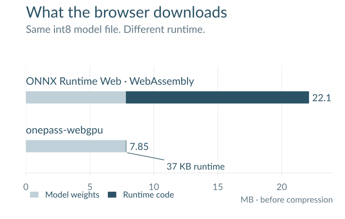
The specialised runtime is roughly 380 times smaller before compression. With gzip, its code is about 12 KB, compared with about 3.7 MB for the reference runtime. Add the 7.8 MB model file to either: shrinking the engine does not make the weights disappear. The comparison demo uses an earlier 24 KB runtime build; the measured 37 KB build also includes direct ONNX loading in the browser.1 The comparison page deliberately loads several engines and both model files so you can time them side by side.
Faster, but does it choose the same move?
For the fp32 path, we checked every one of the 17 325 evaluation positions through the demo's own encoding and runtime path. All 17 325 chosen columns matched the ONNX Runtime fp32 reference. Scores differed slightly, with a largest absolute difference of about 0.000066. Using fp16 weights changed three choices, on positions with nearly tied scores.5
The int8 path needs a more careful description. The same compressed file can be executed with different arithmetic. ONNX Runtime dynamically quantizes intermediate activations as well as using the quantized weights. Our WebGPU path keeps the weights packed as eight-bit values, unpacks them inside the matrix multiplication and computes with float32 activations.
It therefore does not always choose the same column as ONNX Runtime's int8 path. It matched its own weight-only reference on all 17 325 positions. Against the original fp32 model, it retained the same choice on 17 128 positions, compared with 17 004 for ONNX Runtime's int8 path. That measures agreement with the original model, not a new game-winning percentage.6
The packed weights also use less GPU memory: about 7.7 MB instead of 29.5 MB in the recorded loading check. This is weight storage, not total browser memory. The largest timing change in the table comes from the runtime and execution path; reducing weight precision is a separate choice.7
The opponent that sometimes thinks for seven seconds
Connect Four already has a smaller, stronger opponent available: an exact solver. Benjamin Rall's MIT-licensed connect-four-ai plays perfectly, and its WebAssembly package is about 1.3 MB including an opening book. For a product whose only job is to offer a good Connect Four opponent, that is a compelling choice.
We put it beside the model in the same browser. After two random opening moves, the solver played both sides optimally, choosing randomly among tied best moves. Across 200 games, we timed 7 652 positions. Each model runtime then scored those exact positions too. The solver kept its search cache within a game and reset it between games.8
| Engine, on the same 7 652 positions | Median | Mean | Slowest |
|---|---|---|---|
| Exact solver, WebAssembly | < 0.1 ms | 40 ms | 6.9 s |
| Model, onepass-webgpu int8 | 1.0 ms | 0.96 ms | 1.3 ms |
| Model, ONNX Runtime WebAssembly int8 | 13.1 ms | 13.1 ms | 13.7 ms |
The solver's typical move was faster than the browser timer could resolve. But its long searches pulled the average up. The model's advantage was a narrow range of turn times, not winning every race.
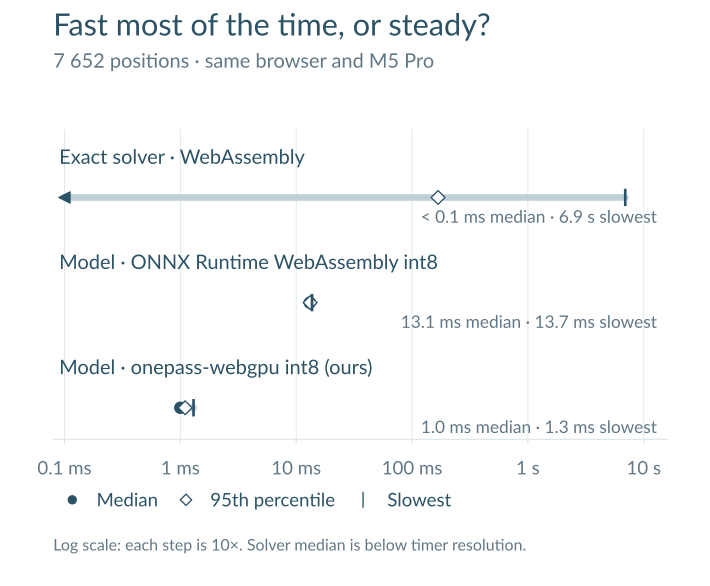
The opening book answers many early positions cheaply, but some positions reached after the random opening moves fall outside it. The slowest search, 6.9 seconds, came with eight or fewer discs on the board. The typical search was longest a little later: at nine to twelve discs, the median was 59 ms. Later still, with few empty cells left, there is little to search.8
The model performs the same fixed-size calculation for every board. That keeps its work predictable, although the device and browser still affect elapsed time. It also gives up the solver's guarantee. The fp32 model selected a move the solver rated best on 91.7% of these positions. That is a different measure from preserving a win or draw, and from winning a whole game.
This is why a solved game makes a useful laboratory. It gives us an answer key for judging a learned decision, even when the eventual application might have no exact solver. Related work by Ruoss and colleagues trained transformers on Stockfish-labelled chess data and obtained grandmaster-level play without explicit search. The expensive teacher does its work before the player needs an answer.9
The GPU that was not a GPU
An early browser run had made WebGPU look painfully slow: hundreds of milliseconds for a move. The adapter turned out to be SwiftShader, a software implementation running on the CPU. We were measuring the cost of pretending to be a GPU.
In that setup, the bundled headless browser had selected the software adapter; installed Chrome in its newer headless mode exposed the real Metal GPU. That is an observation about our test environment, not a rule that headless browsers always use software. The runtime now checks the adapter and refuses recognised software implementations by default.10
Lesson learned: Before explaining a surprising performance number, find out what ran it.
From MLX weights to browser kernels
There are two things to carry from training into a browser: the learned numbers and the instructions for using them. They travel together in the ONNX file, but they take different paths once it arrives.
We trained with MLX on Apple silicon, copied the weights through NumPy into a matching PyTorch model, checked their outputs and exported ONNX from PyTorch. The exporter checks selected moves against ONNX Runtime too.11
| Stage | What crosses the boundary |
|---|---|
| MLX → PyTorch | Parameters with matching names and shapes |
| PyTorch → ONNX | Graph, weights and input/output definitions |
| ONNX + plan → runtime | Layer configuration and weight arrays |
| Runtime → WebGPU | Buffers, compute pipelines and dispatches |
| WebGPU → game | Seven float32 scores, one per option slot |
In the measured runs and demo, a small Python compiler recognises the layers
ahead of time and writes a plan: a few kilobytes of JSON naming the weights and
configuring the kernels. The browser reads the weights from the unchanged ONNX
file and uploads them to GPU buffers. The newer 37 KB build can also recognise
the graph in the browser with Engine.fromOnnx; its tests produce the same plan
for all three published model files. Loading is done once, not for every
move.2
The ONNX file supplies the model; the runtime supplies the GPU programs that
execute it. We are not automatically translating each ONNX node into a shader.
The supported patterns select hand-written kernels from
runtime/src/kernels.ts.
The browser compiles the WGSL for the native GPU backend, Metal on these Macs. The runtime creates and caches its pipelines during loading for single moves, then reuses them. Browser and driver compilation details remain implementation choices; the reported timings are warmed.12
For a builder using the newer direct loader, the API looks like this:
import { Engine } from "./onepass-webgpu.js";

const bytes = await (await fetch("onepass-c4-v2-int8.onnx")).arrayBuffer();
const engine = await Engine.fromOnnx(bytes);
await engine.wake();
const scores = await engine.score(contextIds, optionIds, optionMask);
The three inputs are Int32Arrays containing the encoded board, column options
and valid-slot mask; scores is a Float32Array with seven values. The
demo's encoder
shows how to prepare them. wake() does a real model run using the existing
buffers. Call it ahead of a decision, as during the disc animation, rather than
counting that extra work as free. We return to that idle-pause problem below.
Each move writes new inputs, then reuses the cached pipelines and dispatch list. A bind group connects a kernel to its buffers; a dispatch specifies how many groups of GPU threads should run. Intermediate activations stay in GPU buffers until the final scores are copied back.
Give a small model enough parallel work
Reaching the real GPU was only the beginning. The first kernels left too much work in long loops handled by too few threads. A GPU can have plenty of arithmetic capacity and still spend its time waiting.
The useful change was to split matrix multiplication along the dimension being summed. More threads work on shorter pieces; the following operation combines their partial results. This is called split-K. Think of dividing a long sum among several people, then adding their subtotals. The extra coordination is worthwhile when the original job leaves most of the team idle.13
Here is the inner loop from the matrix-multiplication kernel, shown with its template choices resolved for ordinary fp32 weights:
for (var kk = 0u; kk < KS; kk += 1u) {
  let w = vec4<f32>(W[wi]);
  wi += stride;
  for (var r = 0u; r < RM; r += 1u) { acc[r] = fma(vec4<f32>(at[r * KS + kk]), w, acc[r]); }
}
KS is only this group's slice of the long sum. Each thread works on four
output columns together through vec4, and fma multiplies and accumulates
their contributions. RM is four rows in the current configuration. The
activation tile at is loaded cooperatively into memory shared by the
workgroup's 64 threads; a barrier makes sure those loads finish before the
loop begins. Other workgroups handle other slices of the sum.
The next operation combines those partial sums while reading its input. In the
feed-forward layers, that input-loading step can also add the bias and apply
ReLU. Other kernels combine the residual addition with the next layer norm, or
sum attention's query, key and value partials while loading them. Combining
these steps avoids separate dispatches just to assemble intermediate results.
The int8 variant changes how w is loaded: four
packed weights are unpacked from a 32-bit word, their zero point is subtracted,
and the scale is applied to the accumulated partial result. The activations
and accumulators remain float32.13
Splitting has a cost: the following operations must read and add more partial sums. Attention repeats that reading for each block of eight queries. The heuristic balances extra parallel work against those reads, keeping at least 32 values of the summed dimension in each split. More splits are not automatically better.13
We tested that tradeoff with the fp32 model on an idle M5 Pro, changing only the split targets. Each setting used the same 500 positions after 20 warm-ups, repeated three times. These are medians across the three runs; GPU time comes from a separate timestamped pass.14
| Split target | Per move | GPU time |
|---|---|---|
| No split | 3.2 ms | 2.82 ms |
| 2 048 | 1.8 ms | 1.51 ms |
| 4 096 (default) | 1.3 ms | 0.98 ms |
| 8 192 | 1.0 ms | 0.72 ms |
With split-K disabled, a move took about 2.5 times as long as at the default
setting. Splitting further reached 1.0 ms on this GPU. The default remains
4 096 until more devices are measured; it is a starting point for tuning, not
an established optimum. The runtime exposes splitTarget and qkvSplitTarget
for that purpose. This experiment changed both together, leaving the model,
precision and kernel code unchanged.14
The runtime also keeps the work together. A move queues 70 small compute jobs in one command buffer, submits it once and reads back only seven scores. In the earlier precision comparison, fp32 GPU time was about 0.92 ms, with warm moves at roughly 1.3 ms. Submission and getting the result back matter at this scale.
With fp16 and int8 weights, GPU time was 0.59 and 0.66 ms; a complete move took 0.9 and 1.0 ms respectively. Those fractions of a millisecond matter less to a player than the int8 file's much smaller download. Lower weight precision does not remove submission and readback costs.1
For an arena evaluating many boards, batching offers another tradeoff. At 64 positions per call, the measured cost per position was 0.32 ms with fp32 weights or 0.24 ms with fp16. That improves throughput, not the wait for one move. The published ONNX graph fixes the batch size at one, so ONNX Runtime Web cannot batch that file; our specialised runtime can. The interactive game needs only one decision at a time.1
In the split-target experiment, all four settings gave about 0.32 ms per position at batch 64. With many boards to process together, splitting the sums brought no measurable throughput benefit in this test.14
For a small, one-position workload, arranging the work can matter more than reducing the number of arithmetic operations.
While you think, the GPU rests
The benchmark asks for hundreds of decisions in a row. A person does not.
In the visible game on an M1 Max, the first move after an idle pause could cost tens of milliseconds more, although GPU timestamps still showed roughly the same compute time. The observed behaviour was consistent with the GPU and its browser process returning from an idle state. A trivial keep-alive submission did not solve it; a real model run did.15
The game already animates a disc dropping into the board. It now uses that interval to warm the model engines, then times the decision after the warm-up has finished. On that M1 Max, the timed move returned to about 5 ms after pauses. The warm-up is extra work, fitted into an existing animation. It is not included in the displayed move time, and it does not turn the entire click-to-move interaction into a one-millisecond operation.16
Measure the pause before the next decision, too. A continuously warm benchmark can miss the very delay a person encounters while using the app.
From a fast number to a useful interaction
We did not retrain the AI model for this result. A runtime built around its particular calculations made warm decisions much faster and removed most of the supporting code download. Checking the choices, the adapter and the first move after a pause made those improvements useful outside the benchmark.
The scope is still small: one model family, with the reported measurements from Chrome on Apple silicon. Other browsers, phones and WebAssembly threading configurations need their own tests. The code, model files, protocol and records are public, so those are experiments another builder can take further.
For Connect Four, the exact solver remains an excellent opponent. The broader possibility is to teach a small model a useful decision, then make that decision fit comfortably into an ordinary application. A game gives us a cheerful place to practise, and a way for you to see the tradeoffs yourself.
The runtime source, demo code and model files are there if you want to follow a move all the way through. How much thinking time does your browser need?
Footnotes
-
Idle M5 Pro speed record, measured 27 September 2026 with runtime
94c8af9. It records each run, model hashes, loaded runtime files, GPU adapter and timing boundaries. Runtime sizes are decimal bytes, excluding model files. The ONNX Runtime JavaScript and WebAssembly total 14 314 404 bytes; onepass-webgpu is 37 464 bytes. Gzip and demo-build context: runtime README. ↩ ↩2 ↩3 ↩4 ↩5 -
Ahead-of-time plan compiler, runtime implementation and browser graph recognition. The benchmark loader uses the prepared plan. Direct ONNX loading is a separately tested path for supported scorer patterns, not general ONNX execution. ↩ ↩2
-
Frozen speed protocol. Correctness checks precede timing. Full evaluation-set parity is a separate check. Chrome's recorded clock resolution is about 0.1 ms; the rounded medians are not microsecond-precision measurements. ↩
-
Microsoft's ONNX Runtime Web performance guidance explains the cross-origin-isolation requirement for multiple WebAssembly threads. The measured pages record
crossOriginIsolated: false. ONNX Runtime is MIT-licensed and serves as the reference implementation here. ↩ -
Full fp32 and fp16 parity record. These checks used Chrome 153 on an M1 Max and the demo's own code path. Matching the selected column does not imply bit-identical scores. ↩
-
Weight-only int8 parity record. Its reference is the NumPy implementation of the execution plan with dequantized weights and float32 arithmetic. The WebGPU and ONNX Runtime int8 paths chose the same column on 17 058 of 17 325 positions. ↩
-
Direct ONNX loading checks, including the exact GPU weight-buffer sizes and separate references for each file. ↩
-
Same-browser, full-game timing record and measurement page. Seed 2026;
connect-four-ai-wasm1.0.0 with its opening book. The solver scores all legal moves, with its cache retained within each game. The 91.7% best-move agreement is for the fp32 WebGPU model; the timing table also includes other execution paths. Model timings are sequential and warmed, without human pauses. This panel is separate from both the 500-position speed protocol and the interactive page's 200-board benchmark. ↩ ↩2 -
Ruoss et al., Amortized Planning with Large-Scale Transformers: A Case Study on Chess, 2024. The authors trained models up to 270 million parameters on Stockfish-labelled positions and reported grandmaster-level blitz play without explicit search. This is related work, not a result of our runtime. ↩
-
Software-adapter rejection and the hardware-adapter rule in the protocol. The software result motivated checking the adapter; it is not included as a valid GPU speed comparison. ↩
-
The public Connect Four recipe's MLX checkpoint conversion and ONNX exporter. The exporter names
context_ids,option_idsandoption_mask, producinglogits; it checks selected moves against the PyTorch model. The optional int8 quantization step follows the fp32 export. ↩ -
The W3C's WGSL shader lifecycle describes shader-module, pipeline and execution stages. Chrome's Dawn implementation includes the Tint WGSL compiler and native GPU backends. Our runtime's pipeline cache is separate from any caching inside the browser or GPU driver. ↩
-
Split-K kernels and partial-result accumulation, alongside command-buffer construction. The public speed record distinguishes GPU timestamps from end-to-end warm latency. ↩ ↩2 ↩3
-
Matched split-target measurement, 28 September 2026. Idle M5 Pro, Chrome 154 with the Metal adapter, fp32 weights and arithmetic. Each row reports the median of three run medians. Warm move timing uses 500 positions per run; GPU timestamps use a separate 200-position pass. Both split targets are varied together; setting both to 1 produces one split per matrix multiplication. The measured revision
9dbc4f3changes only the benchmark harness relative to the article's pinned runtime. This isolates the current split settings, not the historical kernel or attention rewrites. ↩ ↩2 ↩3 -
Idle-pause probe and the runtime's warm-up guidance. These development observations concern an M1 Max in a visible Chrome window; they are not the idle M5 Pro benchmark results. ↩
-
Disc animation and engine warm-up in the demo. The page checks reference outputs before trusting the WebGPU player and falls back to WebAssembly if that check fails. Its interactive numbers depend on the reader's device and the page's own position selection. ↩